


-
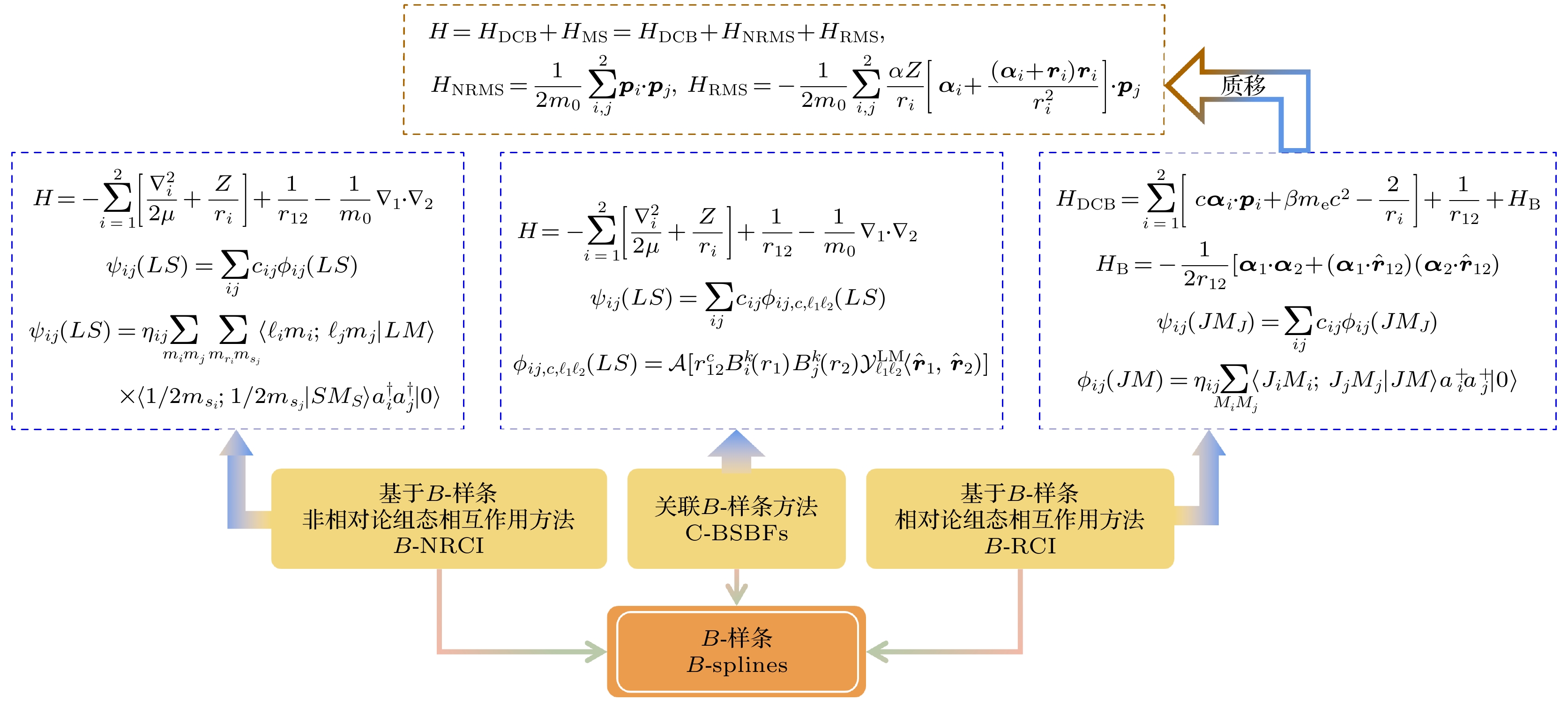
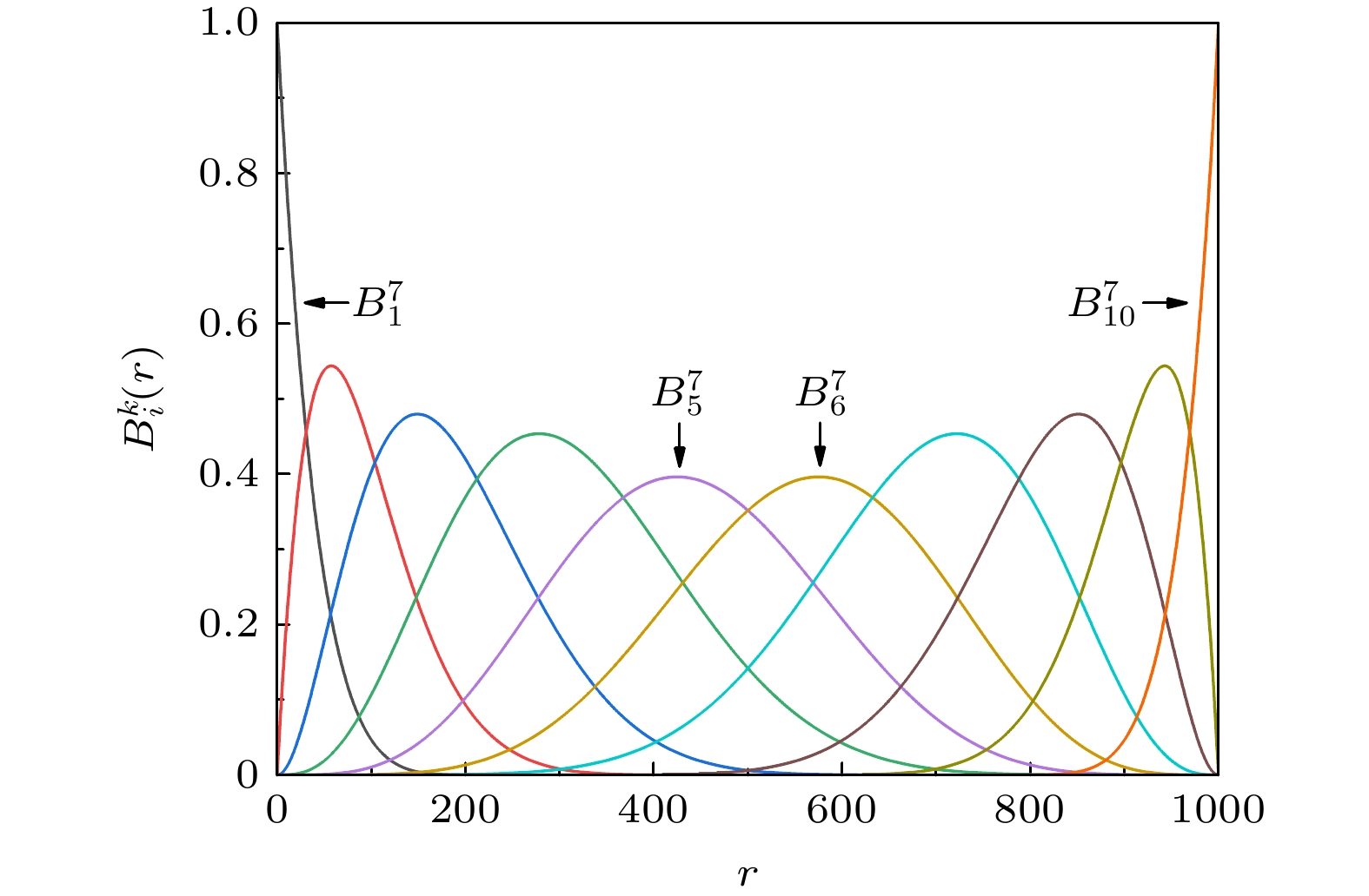
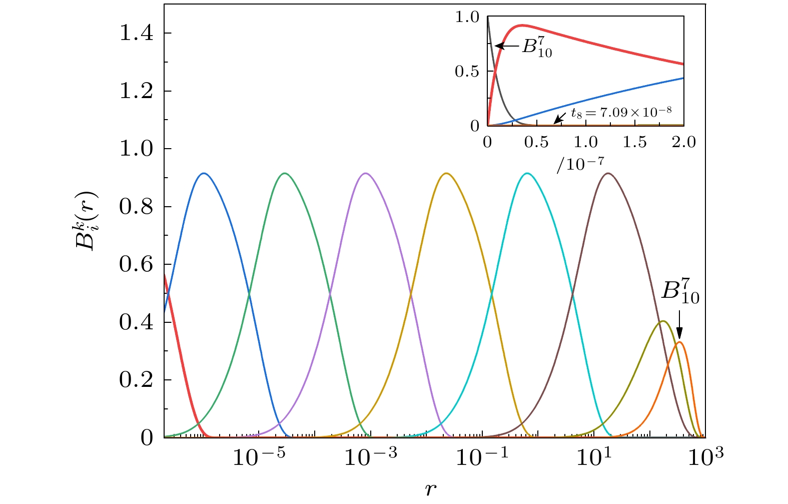
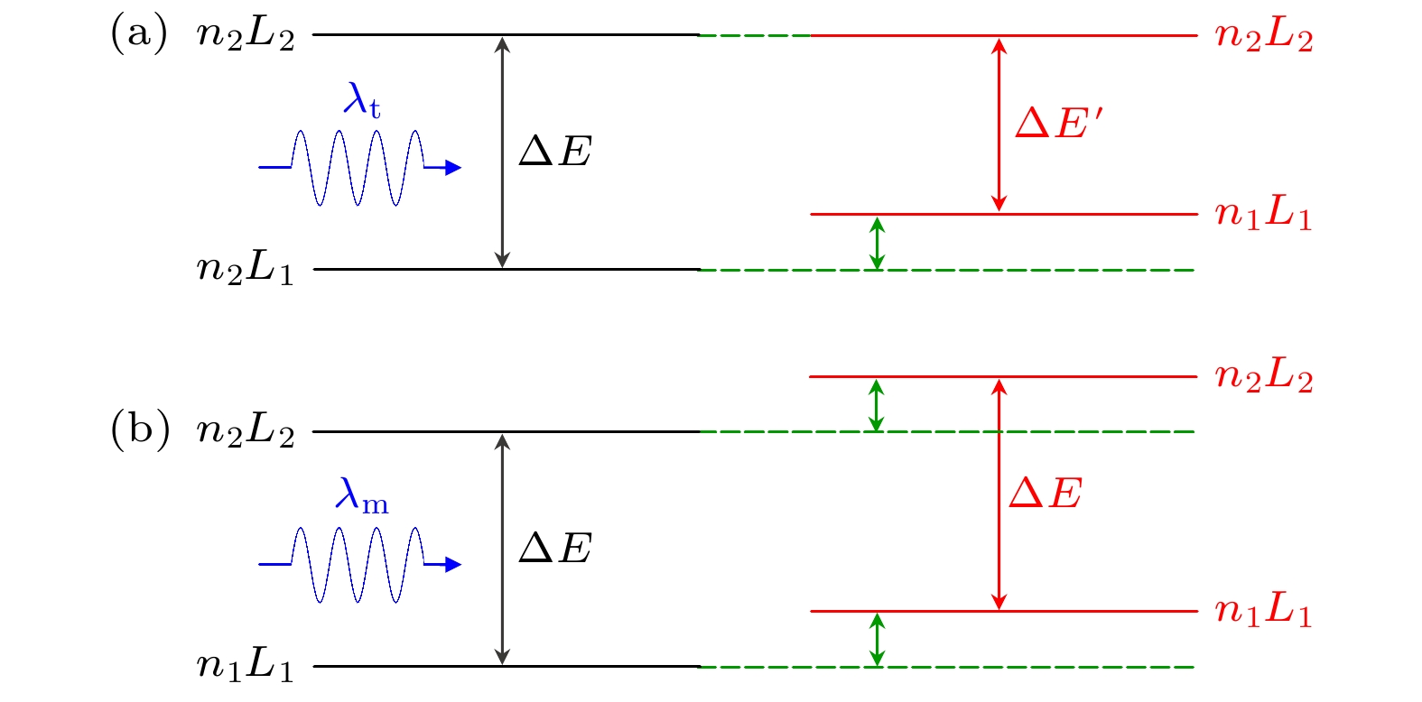
The precise spectra of few-electron atoms plays a pivotal role in advancing fundamental physics, including the verification of quantum electrodynamics (QED) theory, the determination of the fine-structure constants, and the exploration of nuclear properties. With the rapid development of precision measurement techniques, the demand for atomic structure data has evolved from simply confirming existence to pursuing unprecedented accuracy. To meet the growing needs for precision spectroscopy experiments, we develop a series of high-precision theoretical methods based on B-spline basis sets, such as the non-relativistic configuration interaction (B-NRCI) method, the correlated B-spline basis functions (C-BSBFs) method, and the relativistic configuration interaction (B-RCI) method. These methods use the unique properties of B-spline functions, such as locality, completeness, and numerical stability, to accurately solve the Schrödinger and Dirac equations for few-electron atoms. Our methods yield significant results, particularly for helium and helium-like ions. Using these methods, we obtain accurate energies, polarizabilities, tune-out wavelengths, and magic wavelengths. Specifically, we achieve high-precision measurements of the energy spectra of helium, providing vital theoretical support for conducting related experimental researches. Additionally, we make high-precision theoretical predictions of tune-out wavelengths, paving the way for new tests of QED theory. Furthermore, we propose effective theoretical schemes to suppress Stark shifts, thereby facilitating high-precision spectroscopy experiments of helium. The B-spline-basis methods reviewed in this paper prove exceptionally effective in high-precision calculations for few-electron atoms. These methods not only provide crucial theoretical support for precision spectroscopy experiments but also pave the new way for testing QED. Their ability to handle large-scale configuration interactions and incorporate relativistic and QED corrections makes them versatile tools for advancing atomic physics research. In the future, the high-precision theoretical methods based on B-spline basis sets are expected to be extended to cutting-edge fields, such as quantum state manipulation, determination of nuclear structure properties, formation of ultracold molecules, and exploration of new physics, thus continuously promoting the progress of precision measurement physics.
-
Keywords:
- B-spline basis sets /
- few-electron atoms /
- polarizabilities /
- Bethe-logarithm
[1] [2] [3] [4] [5] [6] [7] [8] [9] [10] [11] [12] [13] [14] [15] [16] [17] [18] [19] [20] [21] [22] [23] [24] [25] [26] [27] [28] [29] [30] [31] [32] [33] [34] [35] [36] [37] [38] [39] [40] [41] [42] [43] [44] [45] [46] [47] [48] [49] [50] [51] [52] [53] [54] [55] [56] [57] [58] [59] [60] [61] [62] [63] [64] [65] [66] [67] [68] [69] [70] [71] [72] [73] [74] [75] [76] [77] [78] [79] [80] [81] [82] [83] [84] [85] [86] [87] [88] [89] [90] [91] [92] [93] [94] [95] [96] [97] [98] -
$ \gamma_0 $ $ t_1 $ $ E_{{\mathrm{max}}} $ $ \beta(1 {\mathrm{s}}) $ 0.005 4.10×10⁻¹ 5.76×10³ 2.258 0.025 2.41×10⁻² 1.59×10⁶ 2.2890 0.035 4.59×10⁻³ 4.32×10⁷ 2.29061 0.045 8.06×10⁻⁴ 1.38×10⁹ 2.290915 0.065 2.17×10⁻⁵ 1.83×10¹³ 2.2909796 0.075 3.43×10⁻⁷ 7.23×10¹⁵ 2.29098109 0.085 5.32×10⁻⁷ 2.96×10¹⁸ 2.290981330 0.105 1.23×10⁻⁹ 5.38×10²⁰ 2.2909813741 0.115 1.84×10⁻¹⁰ 2.36×10²² 2.29098137505 0.125 2.74×10⁻¹⁰ 1.05×10²³ 2.29098137518 0.135 4.04×10⁻¹¹ 4.75×10²³ 2.2909813752020 0.145 5.94×10⁻¹² 2.16×1025 2.29098137520502 0.165 1.26×10⁻¹³ 4.65×1028 2.290981375205541 0.175 1.83×10⁻¹⁴ 2.17×1030 2.2909813752055506 0.185 2.65×10⁻¹⁵ 1.03×1032 2.29098137520555206 0.195 3.82×10⁻¹⁶ 4.86×1033 2.29098137520555227 0.205 5.49×10⁻¹⁷ 2.32×1035 2.290981375205552296 0.225 1.13×10⁻¹⁸ 5.35×1038 2.29098137520555230124 0.235 1.60×10⁻¹⁹ 6.31×1039 2.2909813752055523013355  DownLoad: CSV
State B-NRCI[65] C-BSBFs[55] Integration method[73] $ 1\, ^1 {\mathrm{S}} $ 4.37034(2) 4.37016022(5) 4.3701602230703(3) 4.37014(2) 4.3701601(1) $ 2\, ^1 {\mathrm{S}} $ 4.36643(1) 4.36641271(1) 4.366412726417(1) 4.366412(1) 4.3664127(1) $ 3\, ^1 {\mathrm{S}} $ 4.369170(1) 4.36916480(6) 4.369164860824(2) 4.3691643(2) 4.3691648(1) $ 4\, ^1 {\mathrm{S}} $ 4.369893(1) 4.36989065(5) 4.369890632356(3) 4.3698903(5) 4.3698906(1) $ 5\, ^1 {\mathrm{S }}$ 4.370152(3) 4.3701520(1) 4.370151796310(4) 4.3701511(2) 4.3701519(1) $ 6\, ^1 {\mathrm{S }}$ 4.37027(1) 4.370267(1) 4.370266974319(5) 4.370266(2) 4.370267(1) $ 7\, ^1{\mathrm{ S}} $ 4.37033(1) 4.370326(1) 4.370325261772(5) 4.37033(1) 4.370326(1)
DownLoad: CSV
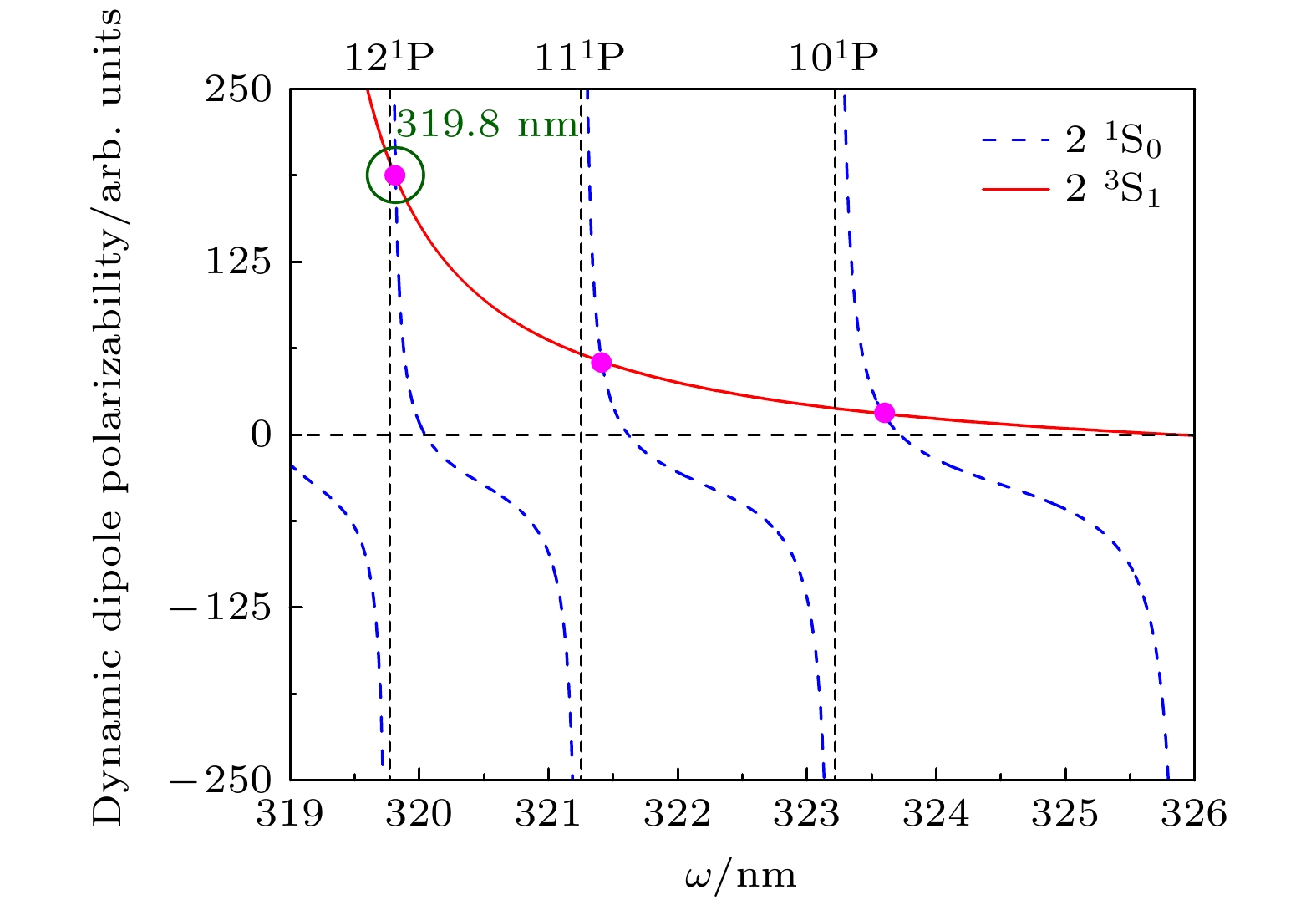
n $ \alpha_1(n\, ^1 {\mathrm{S}}_0) $ $ \alpha_1^{\mathrm{S}}(n\, ^3 {\mathrm{S}}_1) $ $ \alpha_1^{\mathrm{T}}(n\, ^3 {\mathrm{S}}_1) $ 2 800.52195(14) 315.728536(48) 0.002764488(2)/0.000726892(6) 3 16890.5275(28) 7940.5494(13) 0.09715509(3)/–0.005470(2) 4 135875.295(23) 68677.988(11) 0.9558(3)/–0.1189(2) 5 669694.55(11) 351945.328(60) 5.2676(2)/–0.7829(3) 6 2443625.15(40) 1315529.52(23) 20.654(3)/–3.291(2) 7 7269026.8(1.2) 3977532.95(69) 64.62(3)/–10.65(3)
DownLoad: CSV
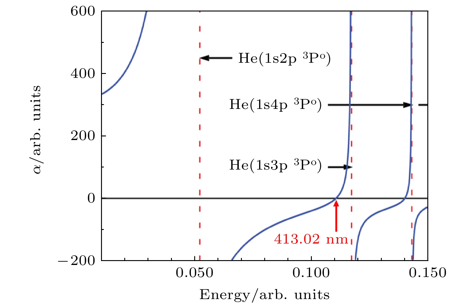
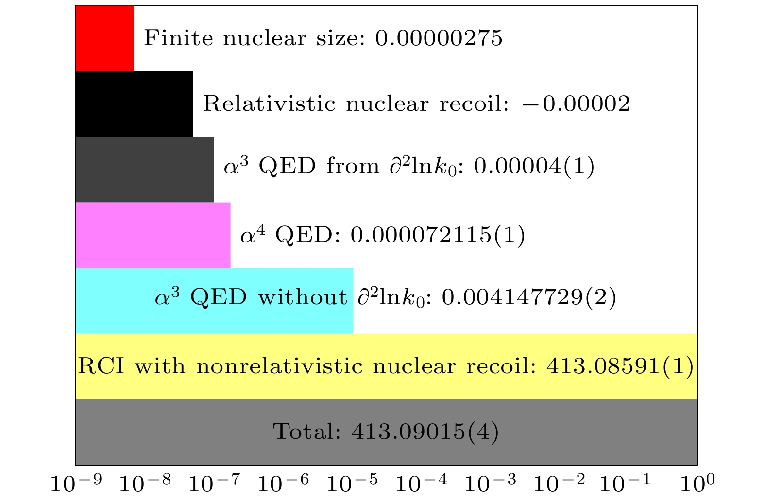
Reference Method $ \alpha_1^{\mathrm{S}}(\omega)-2\alpha_1^{\mathrm{T}}(\omega) $ $ \alpha_1^{\mathrm{S}}(\omega)+\alpha_1^{\mathrm{T}}(\omega) $ $ \alpha_1^{\mathrm{S}}(\omega)-\tfrac{1}{2}\alpha_1^{\mathrm{T}}(\omega) $ Ref. [6] Hybrid model 413.02(9) Ref. [89] Expt. 413.0938(9stat)(20syst) Ref. [47] RCI 413.080 1(4) 413.085 9(4) Ref. [49] RCI+NRQED 413.084 26(4) 413.090 15(4) Ref. [15] Expt. 413.087 08(15) Ref. [15] NRQED 413.087 179(6) Ref. [90] RCIRP 413.084 28(5) 413.090 17(3) 413.087 23(3)
DownLoad: CSV
-
[1] [2] [3] [4] [5] [6] [7] [8] [9] [10] [11] [12] [13] [14] [15] [16] [17] [18] [19] [20] [21] [22] [23] [24] [25] [26] [27] [28] [29] [30] [31] [32] [33] [34] [35] [36] [37] [38] [39] [40] [41] [42] [43] [44] [45] [46] [47] [48] [49] [50] [51] [52] [53] [54] [55] [56] [57] [58] [59] [60] [61] [62] [63] [64] [65] [66] [67] [68] [69] [70] [71] [72] [73] [74] [75] [76] [77] [78] [79] [80] [81] [82] [83] [84] [85] [86] [87] [88] [89] [90] [91] [92] [93] [94] [95] [96] [97] [98]


 DownLoad:


Catalog
Metrics
- Abstract views: 425
- PDF Downloads: 12
- Cited By: 0