


-
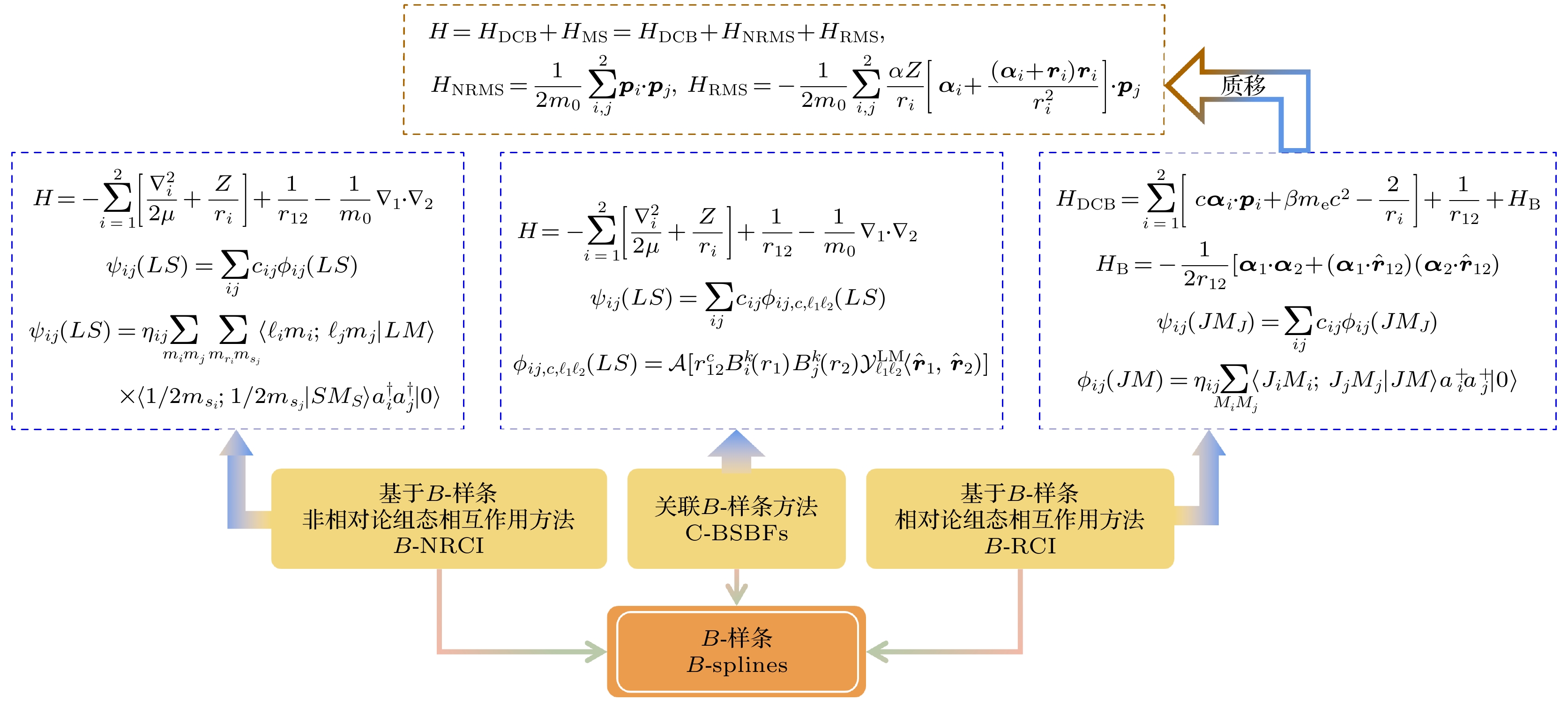
少电子原子的精密光谱在基本物理理论验证、精细结构常数精确测定以及原子核性质深入探索等领域具有重要的应用价值. 随着精密测量物理学的快速发展, 人们对原子结构数据的需求已从最初的存在性确认, 转变为对高度准确性和精确性的持续追求. 为了满足精密光谱实验对高精度结构性质数据的迫切需求, 我们自主发展了一系列基于B-样条基组的高精度理论方法, 并将其成功应用于少电子原子的能级结构与外场响应性质的理论研究中. 具体而言, 实现了氦原子和类氦离子能谱的高精度确定, 为相关实验研究提供理论支撑; 实现了幻零波长的高精度理论预言, 为量子电动力学理论检验开辟了新方向; 提出了有效抑制光频移的理论方案, 为氦原子高精度光谱实验的开展提供了重要支持. 展望未来, 基于B-样条基组的高精度理论方法有望在量子态操控、核结构性质精确测定、超冷分子形成以及新物理探索等前沿领域得到广泛应用, 从而推动国内外精密测量物理领域的蓬勃发展.The precise spectra of few-electron atoms plays a pivotal role in advancing fundamental physics, including the verification of quantum electrodynamics (QED) theory, the determination of the fine-structure constants, and the exploration of nuclear properties. With the rapid development of precision measurement techniques, the demand for atomic structure data has evolved from simply confirming existence to pursuing unprecedented accuracy. To meet the growing needs for precision spectroscopy experiments, we develop a series of high-precision theoretical methods based on B-spline basis sets, such as the non-relativistic configuration interaction (B-NRCI) method, the correlated B-spline basis functions (C-BSBFs) method, and the relativistic configuration interaction (B-RCI) method. These methods use the unique properties of B-spline functions, such as locality, completeness, and numerical stability, to accurately solve the Schrödinger and Dirac equations for few-electron atoms. Our methods yield significant results, particularly for helium and helium-like ions. Using these methods, we obtain accurate energies, polarizabilities, tune-out wavelengths, and magic wavelengths. Specifically, we achieve high-precision measurements of the energy spectra of helium, providing vital theoretical support for conducting related experimental researches. Additionally, we make high-precision theoretical predictions of tune-out wavelengths, paving the way for new tests of QED theory. Furthermore, we propose effective theoretical schemes to suppress Stark shifts, thereby facilitating high-precision spectroscopy experiments of helium. The B-spline-basis methods reviewed in this paper prove exceptionally effective in high-precision calculations for few-electron atoms. These methods not only provide crucial theoretical support for precision spectroscopy experiments but also pave the new way for testing QED. Their ability to handle large-scale configuration interactions and incorporate relativistic and QED corrections makes them versatile tools for advancing atomic physics research. In the future, the high-precision theoretical methods based on B-spline basis sets are expected to be extended to cutting-edge fields, such as quantum state manipulation, determination of nuclear structure properties, formation of ultracold molecules, and exploration of new physics, thus continuously promoting the progress of precision measurement physics.
-
Keywords:
- B-spline basis sets /
- few-electron atoms /
- polarizabilities /
- Bethe-logarithm
[1] [2] [3] [4] [5] [6] [7] [8] [9] [10] [11] [12] [13] [14] [15] [16] [17] [18] [19] [20] [21] [22] [23] [24] [25] [26] [27] [28] [29] [30] [31] [32] [33] [34] [35] [36] [37] [38] [39] [40] [41] [42] [43] [44] [45] [46] [47] [48] [49] [50] [51] [52] [53] [54] [55] [56] [57] [58] [59] [60] [61] [62] [63] [64] [65] [66] [67] [68] [69] [70] [71] [72] [73] [74] [75] [76] [77] [78] [79] [80] [81] [82] [83] [84] [85] [86] [87] [88] [89] [90] [91] [92] [93] [94] [95] [96] [97] [98] -
$ \gamma_0 $ $ t_1 $ $ E_{{\mathrm{max}}} $ $ \beta(1 {\mathrm{s}}) $ 0.005 4.10×10⁻¹ 5.76×10³ 2.258 0.025 2.41×10⁻² 1.59×10⁶ 2.2890 0.035 4.59×10⁻³ 4.32×10⁷ 2.29061 0.045 8.06×10⁻⁴ 1.38×10⁹ 2.290915 0.065 2.17×10⁻⁵ 1.83×10¹³ 2.2909796 0.075 3.43×10⁻⁷ 7.23×10¹⁵ 2.29098109 0.085 5.32×10⁻⁷ 2.96×10¹⁸ 2.290981330 0.105 1.23×10⁻⁹ 5.38×10²⁰ 2.2909813741 0.115 1.84×10⁻¹⁰ 2.36×10²² 2.29098137505 0.125 2.74×10⁻¹⁰ 1.05×10²³ 2.29098137518 0.135 4.04×10⁻¹¹ 4.75×10²³ 2.2909813752020 0.145 5.94×10⁻¹² 2.16×1025 2.29098137520502 0.165 1.26×10⁻¹³ 4.65×1028 2.290981375205541 0.175 1.83×10⁻¹⁴ 2.17×1030 2.2909813752055506 0.185 2.65×10⁻¹⁵ 1.03×1032 2.29098137520555206 0.195 3.82×10⁻¹⁶ 4.86×1033 2.29098137520555227 0.205 5.49×10⁻¹⁷ 2.32×1035 2.290981375205552296 0.225 1.13×10⁻¹⁸ 5.35×1038 2.29098137520555230124 0.235 1.60×10⁻¹⁹ 6.31×1039 2.2909813752055523013355  下载: 导出CSV
State B-NRCI[65] C-BSBFs[55] Integration method[73] $ 1\, ^1 {\mathrm{S}} $ 4.37034(2) 4.37016022(5) 4.3701602230703(3) 4.37014(2) 4.3701601(1) $ 2\, ^1 {\mathrm{S}} $ 4.36643(1) 4.36641271(1) 4.366412726417(1) 4.366412(1) 4.3664127(1) $ 3\, ^1 {\mathrm{S}} $ 4.369170(1) 4.36916480(6) 4.369164860824(2) 4.3691643(2) 4.3691648(1) $ 4\, ^1 {\mathrm{S}} $ 4.369893(1) 4.36989065(5) 4.369890632356(3) 4.3698903(5) 4.3698906(1) $ 5\, ^1 {\mathrm{S }}$ 4.370152(3) 4.3701520(1) 4.370151796310(4) 4.3701511(2) 4.3701519(1) $ 6\, ^1 {\mathrm{S }}$ 4.37027(1) 4.370267(1) 4.370266974319(5) 4.370266(2) 4.370267(1) $ 7\, ^1{\mathrm{ S}} $ 4.37033(1) 4.370326(1) 4.370325261772(5) 4.37033(1) 4.370326(1)
下载: 导出CSV
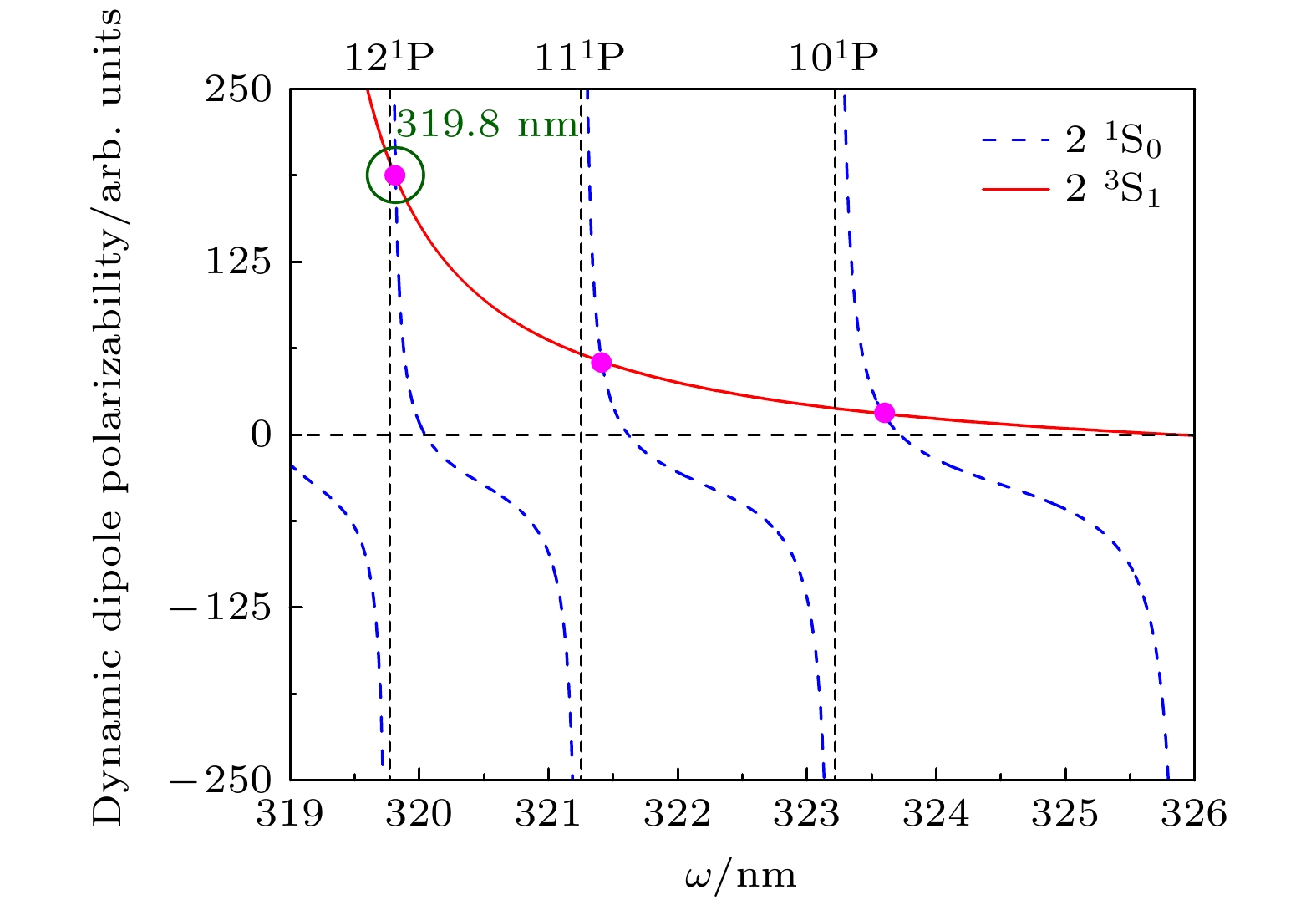
n $ \alpha_1(n\, ^1 {\mathrm{S}}_0) $ $ \alpha_1^{\mathrm{S}}(n\, ^3 {\mathrm{S}}_1) $ $ \alpha_1^{\mathrm{T}}(n\, ^3 {\mathrm{S}}_1) $ 2 800.52195(14) 315.728536(48) 0.002764488(2)/0.000726892(6) 3 16890.5275(28) 7940.5494(13) 0.09715509(3)/–0.005470(2) 4 135875.295(23) 68677.988(11) 0.9558(3)/–0.1189(2) 5 669694.55(11) 351945.328(60) 5.2676(2)/–0.7829(3) 6 2443625.15(40) 1315529.52(23) 20.654(3)/–3.291(2) 7 7269026.8(1.2) 3977532.95(69) 64.62(3)/–10.65(3)
下载: 导出CSV
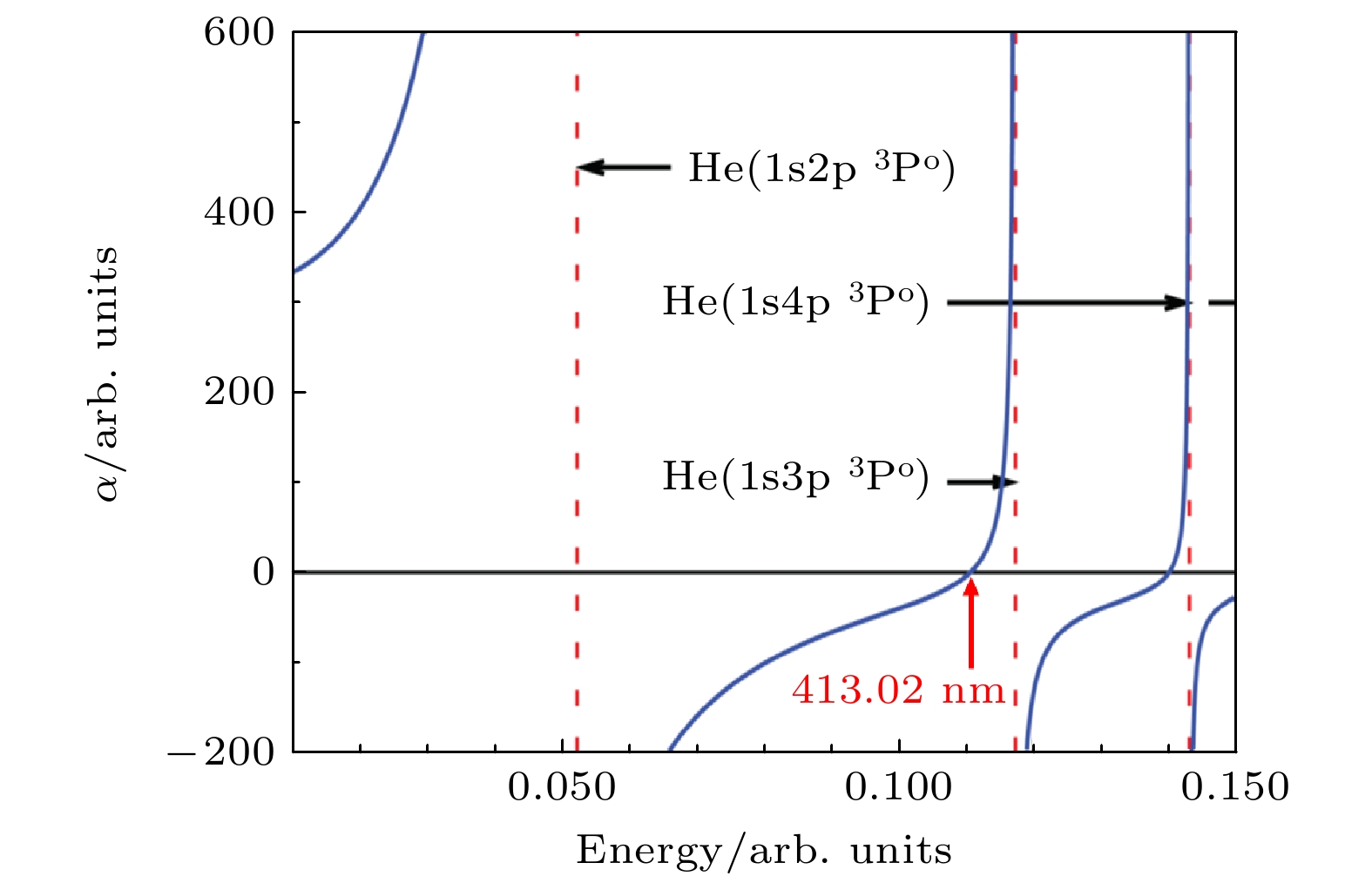
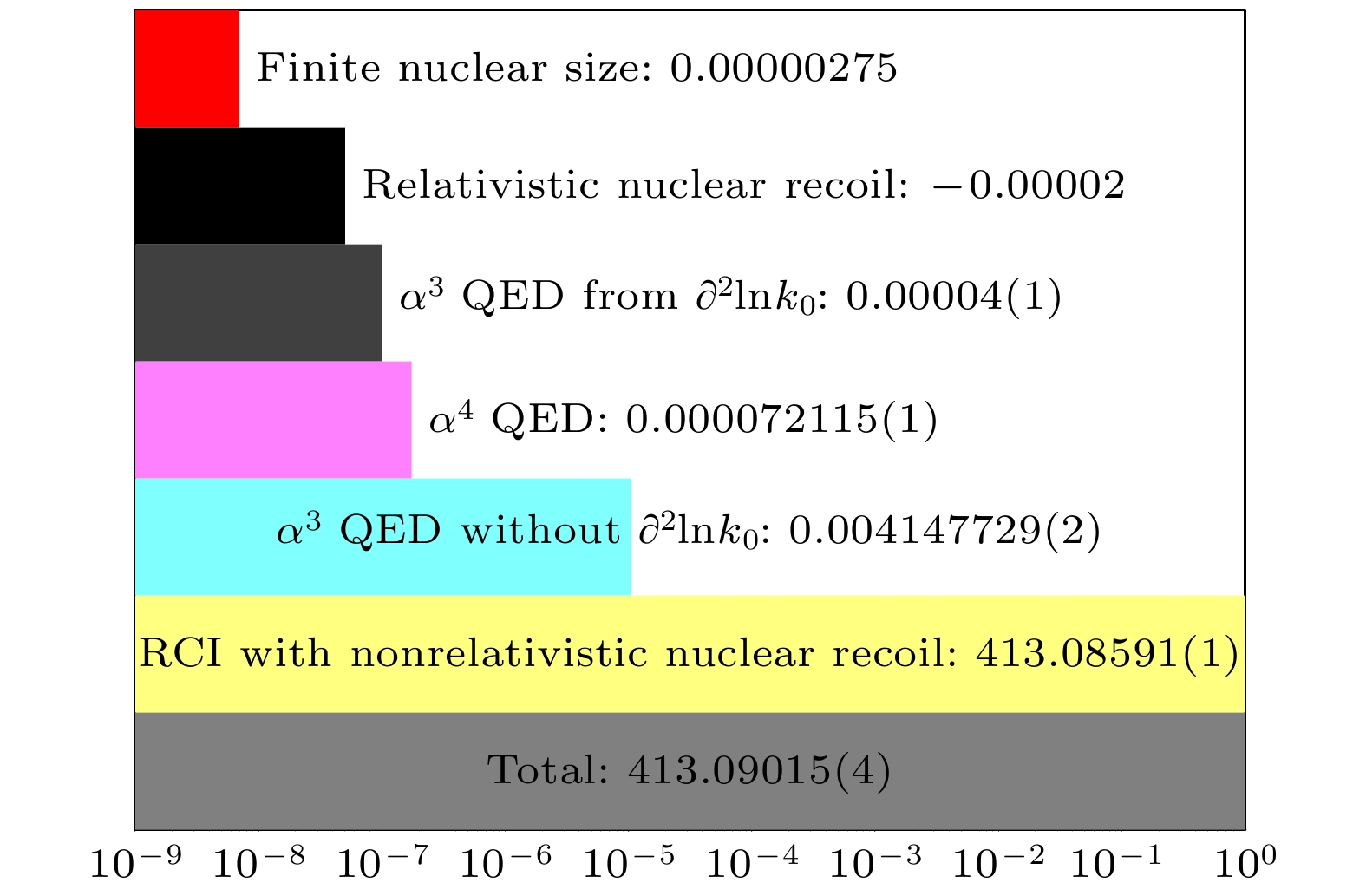
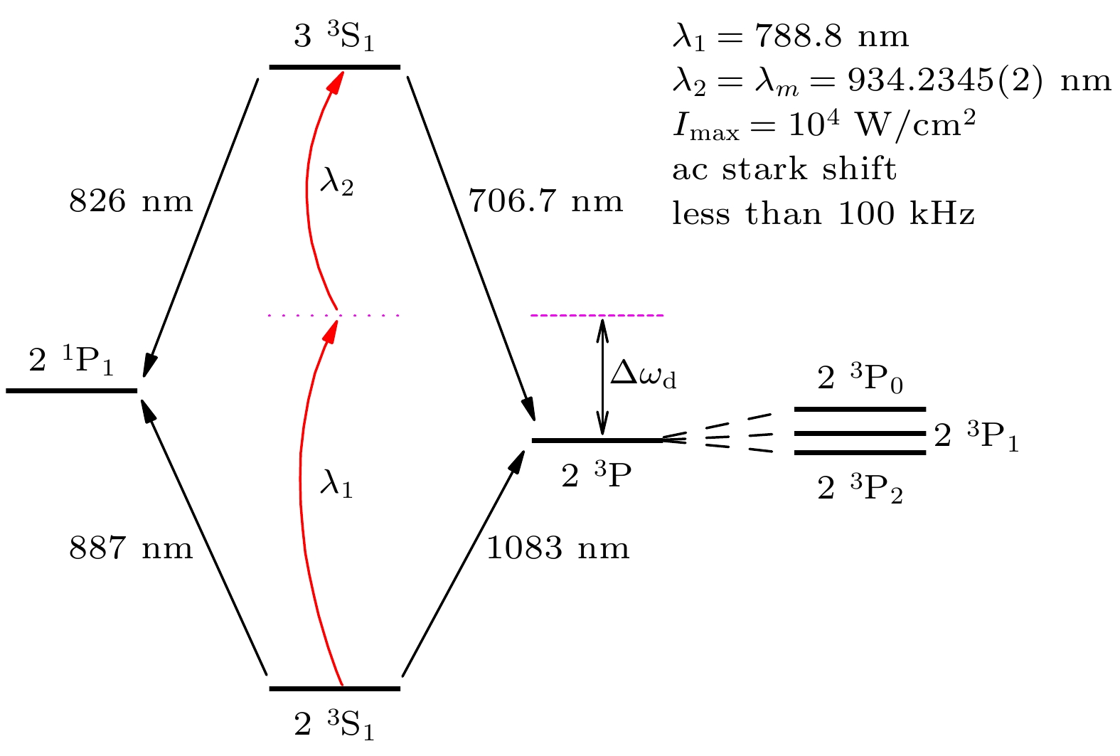
Reference Method $ \alpha_1^{\mathrm{S}}(\omega)-2\alpha_1^{\mathrm{T}}(\omega) $ $ \alpha_1^{\mathrm{S}}(\omega)+\alpha_1^{\mathrm{T}}(\omega) $ $ \alpha_1^{\mathrm{S}}(\omega)-\tfrac{1}{2}\alpha_1^{\mathrm{T}}(\omega) $ Ref. [6] Hybrid model 413.02(9) Ref. [89] Expt. 413.0938(9stat)(20syst) Ref. [47] RCI 413.080 1(4) 413.085 9(4) Ref. [49] RCI+NRQED 413.084 26(4) 413.090 15(4) Ref. [15] Expt. 413.087 08(15) Ref. [15] NRQED 413.087 179(6) Ref. [90] RCIRP 413.084 28(5) 413.090 17(3) 413.087 23(3)
下载: 导出CSV
-
[1] [2] [3] [4] [5] [6] [7] [8] [9] [10] [11] [12] [13] [14] [15] [16] [17] [18] [19] [20] [21] [22] [23] [24] [25] [26] [27] [28] [29] [30] [31] [32] [33] [34] [35] [36] [37] [38] [39] [40] [41] [42] [43] [44] [45] [46] [47] [48] [49] [50] [51] [52] [53] [54] [55] [56] [57] [58] [59] [60] [61] [62] [63] [64] [65] [66] [67] [68] [69] [70] [71] [72] [73] [74] [75] [76] [77] [78] [79] [80] [81] [82] [83] [84] [85] [86] [87] [88] [89] [90] [91] [92] [93] [94] [95] [96] [97] [98]

 下载:
下载:
计量
- 文章访问数: 428
- PDF下载量: 12
- 被引次数: 0